Simple Linear Regression

Linear Regression is a statistical approach to modeling the relationship between a scalar response(dependent variable) and one or more explanatory variables(independent variables). It is one of the most basic and studied forms of regression analysis and in machine learning, it is one of the fundamental supervised algorithms. A simple Linear Regression would be between a dependent variable and an independent variable.

In this post, I will try to explain some of the concepts of Linear Regression using examples and having a working model in Python.

Contents:

• The concept of Linear Regression.
• Cost Function. A bit of mathematical inference of the Cost Function.
• Gradient Descent!
• Working out an LR example.
• Conclusion and Resources.

Notation:

The following notations will be used throughout this post, and in cases of minor changes, I shall do well to state an eleborate description as to how and why, otherwise:

$X$ - training input(Features)

$y$ - training output(Target)

$(X,y)$ - A sample of Training set

$(X^{i}, y^{i})$ - ith batch of training set

$n$ - Number of training features $(X)$

$m$ - Number of training examples

$\theta_{i}$ - Parameters of our Hypothesis.

The Concept of Linear Regression.

The construct below shows the underlying concept of Linear regression; given a set of predictors $X$ and an outcome $y$, we fit a straight line that not only explains the data but also serves as a predictive model for unseen data.

There are quite a number of assumptions to consider when using linear regression to predict outputs. However, we would be discussing the most common ones:

• Separability/additivity: It's a very big assumption that plays on the effects of things in isolation add up when they happen together. In layman's terms, If there exist multiple pieces of information that would affect the outcome of the prediction, each of the available information could be summed up as if they were being used in isolation.

• Monotonicity/linearity: A monotonic model is one where changing one of the inputs has a corresponding change(up or down) in the response variable. It assumes as the explanatory variables increase so should the outcome, which isn't always true. Thus, monotonicity holds less compared to the linearity of a model, which is merely a restriction on the parameters(regression coefficients), and speaks loudly of the linear relationship between the mean of the response variable and the explanatory variables.

• Lack of perfect multicollinearity in the predictors.

Cost Function

Put simply,

The cost function is a measure of how wrong the model is in terms of its ability to estimate the relationship between X and y.

Before delving into the cost function, let's shine some light on the Hypothesis, a parametric responsibe for getting the best function(i.e, the best line) that explains $X$ and $y$

Hypothesis: $h_{\theta}(x) = \theta_{0} + \theta_{1} X_{1} + \theta_{2} X_{2}+ ... + \theta_{n} X_{n} \label{a}\tag{1}$

Or, in our case, a SLR: $h_{\theta}(x) = \theta_{0} + \theta_{1} x + \epsilon\tag{2}$

where $\epsilon = \left\lvert y - h_{\theta}(x) \right\rvert$

$h_{\theta}(x) = \theta_{1} x\tag{3}$

Taking $\theta_{0}$ to be 0. That is, our intercept goes through the origin, as seen below.

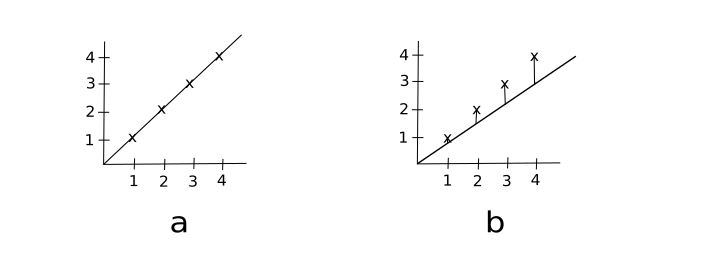
We can clearly see (a) is the best fit with $\theta_{1}$ given as 1. Here's how:

Calculations:

Our training features, in vector notation: $X \epsilon \mathbb{R}^{4 \times 1}$

The term $(\frac {1}{2m})$ below is added for convenience, so we can calculate our gradient(slope) in a much more interpretable fashion. $m$ is the size of our data, and in this case, 4.

Now, let's manually try getting $\theta_{1}$ that minimizes the cost function.

(a) Randomly picked, $\theta_{1}$ is 1.

i. Cost Function: $J(\theta_{1}) = (\frac{1}{2m}) \sum_{i=1}^{m}\left\lvert(h(x)^{i} - y^{i})\right\rvert^2$

ii. $J(\theta_{1}) = (\frac{1}{2m}) \sum_{i=1}^{m}( (\theta_{i} x^{i} - y^{i}) )^2$

iii. $J(\theta_{1}) = (\frac{1}{2 \times 4}) ( 0^2 + 0^2 + 0^2 + 0^2 )$, which gives us 0.

(b) Randomly picked, $\theta_{1}$ is 0.8.

i. $J(\theta_{1}) = (\frac{1}{2 \times 4}) |(0.8 - 1)^2 + (1.5 - 2)^2 + (2.2 - 3)^2 + (2.8 - 4) ^2 |$

ii. $J(\theta_{1}) = (\frac{1}{2 \times 4}) (2.37)$

iii. $J(\theta_{1}) = (\frac{2.37}{8})$, which gives us 0.296.

Cost Function graph, after trying other arbitary values for $\theta_{1}$:

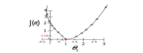
So, what's the value of $\theta_{1}$ that minimizes $J(\theta_{1})$? Yeah? ONE! (CF is 0 when $\theta_{1}$ is 1 and 0.296 at a value of 0.8). You can tell just by eyeballing the graph.

IMPORTANT:

• In actual practice, you'd be dealing with more than one weight and while you can manually compute your weights(parameters, $\theta$) either by brute-forcing or random-guessing, it's never really a good idea to do so as it can be something of a computational nightmare.

• In general, the cost function is often represented as: $$J(\theta) = (\frac{1}{2}) \sum_{i=1}^{m}\left\lvert(h(x)^{i} - y^{i})\right\rvert^2$$

Gradient Descent

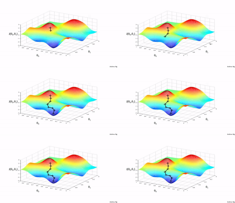
Gradient Descent is an optimization algorithm that aids in finding the right parameters($\theta s$) that minimize the cost function. Say we have a cost function, $J(\theta_0,\theta_1) = (\frac{1}{m}) \sum_{i=1}^{m} \left| \left(h(x)_i - y_i \right)^2\right| \label{e}$ and we need to minimize it, to get the best fit for our training data, Gradient Descent goes through a routine of finding the "right" $\theta s$ to achieve that.

Gradient Descent, in non-zorgon: Mary's lamb is at the bottom of a mountain, the minimum. Mary would very much like to get to her helpless lamb from the mountain top. Mary has a plan. And it is a simple plan; go down the mountain at a steady pace($\alpha$, learning rate), but how would a blindfolded Mary tell what way's down? She came up with the idea of feeling her environment(gradient/slope) until she gets to her lamb at the bottom.

Mathematically,

repeat until convergence { $\theta_{j} := \theta_{j} - \alpha \frac{\partial}{\partial \theta_{j}}J(\theta_{0}, \theta_{1})$ (for j = 0 and j = 1) }

And the update is done as follow, simultaneously:

temp 0 $:= \theta_{0} - \alpha \frac{\partial}{\partial \theta_{j}}J(\theta_{0}, \theta_{1})$
temp 1 $:= \theta_{1} - \alpha \frac{\partial}{\partial \theta_{j}}J(\theta_{0}, \theta_{1})$

$\theta_{0} := temp0$
$\theta_{1} := temp1$

Concept of the Gradient Descent:

1. Start with some $\theta_{0},\theta_{1}$ (e.g., $\theta_{0} = 0, \theta_{1} = 0$)
2. Keep updating $\theta_{0},\theta_{1}$ to reduce the cost function $J(\theta_0, \theta_1)$ until we end up at a minimum.

Graphically,

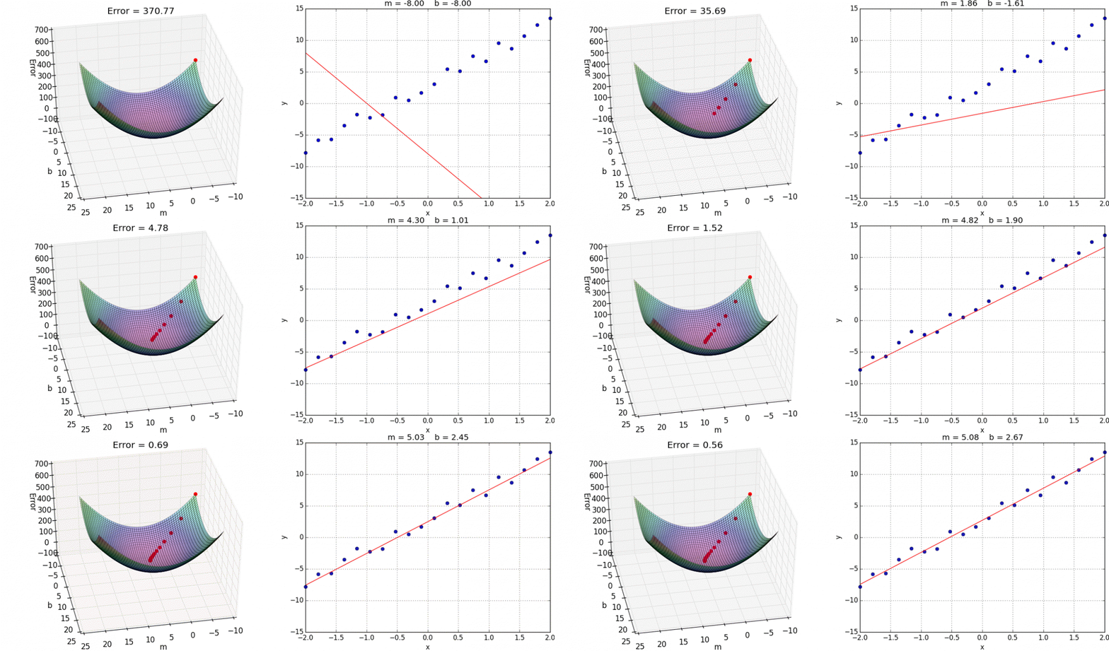source: hackernoon

Where $b$ and $m$ could be represented as $\theta_{0}$ and $\theta_{1}$ respectively, as in our graph.

IMPORTANT!: Finding the minima(local or global) step-wise isn't completely dependent on $\alpha$ as the gradient(slope) itself plays a major role. The weight(s), from the slope's calculations, goes against the negative gradient and keeps moving until reaching minima. Also, worthy of note:

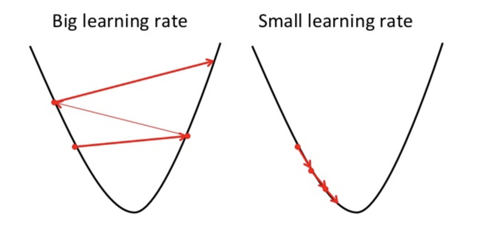
• If the value of $\alpha$ is too small, gradient descent can be slow.
• If $\alpha$ is too large, gradient descent can overshot the minimum, failing to converge, or even diverge.

• If you are already at a global minimum, $\theta_{n}$ is unchanged, i.e., $$ \begin{array}{c} \theta_{n} := \theta_{n} - \alpha \times 0\ \theta_{n} := \theta_{n} - 0\ \theta_{n} := \theta_{n}\ \end{array} $$

Working out an example:

In [1]:

import matplotlib.pyplot as plt
%matplotlib inline



X = [[17], [20], [13], [22], [30], [32], [25]] #Age
y = [[45], [51], [48], [58], [62], [60], [58]] #Weight
plt.figure()
plt.title('Age plotted against weight.')
plt.xlabel('Age')
plt.ylabel('Weight (in kg)')
plt.plot(X, y, 'k.')
plt.axis([10, 40, 30, 70])
plt.grid(True)
plt.show()

from sklearn.linear_model import LinearRegression
lr= LinearRegression()

X = [[17], [20], [13], [22], [30], [32], [25]] #Age
y = [[45], [51], [48], [58], [62], [60], [58]] #Weight

lr.fit(X,y) #learn the parameters

LinearRegression(copy_X=True, fit_intercept=True, n_jobs=None,
         normalize=False)

In [3]:

plt.scatter(X,y)
plt.plot(X, lr.predict(X), color='k')
plt.axis([10, 40, 30, 70])

Out[3]:

[10, 40, 30, 70]

print("A 40 year old should weight about: {} (in Kg)".format(lr.predict([[40],])))

A 40 year old should weight about: [[69.30316973]] (in Kg)

lr.coef_ #$\theta_{1}$

array([[0.85224949]])

Conclusion

Linear regression models are a good starting point for regression tasks and while this is an overview of a Simple Linear Regression, do take note that implementations of the regression technique are beyond the scope of what you've seen to this point.

I had hoped this would contain as much math as I would like but I'm quite ok with the content. In practice, it requires a lot of math to really understand the fundamentals.

Resources

1. Mastering Machine Learning with scikit-learn (by Gavin Hackeling)
2. Andrew NG's course on Machine Learning.
3. Wikipedia - Linear Regression